4 Easy Facts About Excel If Formula Described

By pushing ctrl+shift+facility, this will determine as well as return value from multiple varieties, as opposed to just individual cells added to or increased by one an additional. Determining the amount, product, or quotient of specific cells is easy-- just utilize the =AMOUNT formula as well as go into the cells, worths, or range of cells you desire to perform that math on.

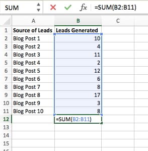
If you're looking to find complete sales revenue from several sold devices, for instance, the array formula in Excel is ideal for you. Below's how you 'd do it: To start utilizing the variety formula, kind "=SUM," as well as in parentheses, enter the very first of 2 (or 3, or 4) varieties of cells you want to increase with each other.

This means multiplication. Following this asterisk, enter your 2nd range of cells. You'll be multiplying this second variety of cells by the very first. Your progress in this formula should now appear like this: =AMOUNT(C 2: C 5 * D 2:D 5) Ready to press Get in? Not so fast ... Because this formula is so complicated, Excel books a different key-board command for ranges.

This will certainly acknowledge your formula as a selection, wrapping your formula in support personalities and also successfully returning your item of both ranges integrated. In earnings computations, this can minimize your effort and time significantly. See the final formula in the screenshot above. The MATTER formula in Excel is denoted =COUNT(Begin Cell: End Cell).

As an example, if there are 8 cells with gotten in worths in between A 1 as well as A 10, =COUNT(A 1: A 10) will return a value of 8. The COUNT formula in Excel is specifically helpful for huge spreadsheets, wherein you intend to see the amount of cells contain real access. Don't be tricked: This formula will not do any type of math on the values of the cells themselves.

The Only Guide for Excel Formulas

Making use of the formula in strong above, you can conveniently run a matter of current cells in your spreadsheet. The outcome will certainly look a little something like this: To carry out the ordinary formula in Excel, enter the values, cells, or variety of cells of which you're calculating the average in the style, =AVERAGE(number 1, number 2, and so on) or =AVERAGE(Begin Value: End Worth).

Discovering the average of a variety of cells in Excel keeps you from needing to find individual sums and after that performing a different division formula on your total amount. Making use of =STANDARD as your initial message access, you can let Excel do all the job for you. For reference, the standard of a group of numbers amounts to the amount of those numbers, divided by the number of products in that group.

This will certainly return the sum of the worths within a desired array of cells that all fulfill one standard. For instance, =SUMIF(C 3: C 12,"> 70,000") would certainly return the amount of values between cells C 3 and also C 12 from just the cells that are greater than 70,000. Allow's state you wish to determine the profit you created from a listing of leads who are related to particular location codes, or compute the amount of certain workers' salaries-- however only if they drop above a certain amount.

With the SUMIF feature, it does not need to be-- you can easily accumulate the sum of cells that satisfy specific standards, like in the income instance above. The formula: =SUMIF(range, criteria, [sum_range] Array: The variety that is being tested using your standards. Requirements: The requirements that figure out which cells in Criteria_range 1 will be combined [Sum_range]: An optional series of cells you're going to accumulate in addition to the very first Array went into.

In the instance below, we desired to compute the amount of the salaries that were greater than $70,000. The SUMIF function accumulated the dollar quantities that surpassed that number in the cells C 3 with C 12, with the formula =SUMIF(C 3: C 12,"> 70,000"). The TRIM formula in Excel is represented =TRIM(text).

6 Simple Techniques For Excel If Formula

For example, if A 2 consists of the name" Steve Peterson" with undesirable rooms prior to the given name, =TRIM(A 2) would certainly return "Steve Peterson" with no areas in a brand-new cell. Email and also file sharing are wonderful devices in today's work environment. That is, until among your associates sends you a worksheet with some actually fashionable spacing.

Rather than meticulously getting rid of and including areas as required, you can clean up any uneven spacing using the TRIM feature, which is used to get rid of additional spaces from data (besides solitary spaces between words). The formula: =TRIM(message). Text: The text or cell where you desire to eliminate areas.

To do so, we entered =TRIM("A 2") right into the Formula Bar, and replicated this for each name listed below it in a brand-new column beside the column with unwanted rooms. Below are some various other Excel formulas you could locate helpful as your data monitoring needs expand. Allow's state you have a line of text within a cell that you wish to damage down right into a few various sectors.

Objective: Utilized to draw out the initial X numbers or personalities in a cell. The formula: =LEFT(message, number_of_characters) Text: The string that you desire to extract from. Number_of_characters: The number of personalities that you wish to extract beginning with the left-most character. In the instance listed below, we went into =LEFT(A 2,4) into cell B 2, as well as copied it right into B 3: B 6.

Purpose: Used to draw out characters or numbers in the middle based on setting. The formula: =MID(message, start_position, number_of_characters) Text: The string that you desire to extract from. Start_position: The placement in the string that you intend to start drawing out from. For example, the first position in the string is 1.

The smart Trick of Learn Excel That Nobody is Discussing

In this example, we entered =MID(A 2,5,2) into cell B 2, and duplicated it right into B 3: B 6. That enabled us to draw out both numbers starting in the fifth placement of the code. Objective: Utilized to draw out the last X numbers or characters in a cell. The formula: =RIGHT(text, number_of_characters) Text: The string that you desire to extract from.

excel formulas y/n formulas excel pdf 2016 excel formula questions and answers pdf